Authors: Jeremy Foote, Aaron Shaw, Benjamin Mako Hill
Archival copies of code and data: https://dx.doi.org/10.7910/DVN/W31PH5
License: see COPYING file: code is released under GNU GPLv3 or any later version; chapter is released as CC BY-NC-SA.
Dramatic increases in large-scale data generated through social media, combined with increased computational power, have enabled the growth of computational approaches to social media research, and social science in general. While many of these approaches require statistical or computational training, they have the great benefit of being inherently transparent—allowing for research that others can reproduce and learn from.
To that end, we wrote a book chapter in the Sage Handbook of Social Media in which we obtain a large-scale dataset of metadata about social media research papers which we analyze using a few commonly-used computational methods. This document is designed to tell you exactly how we did that and to walk you through how to reproduce our results and our paper by running the code we wrote.
This document is meant to be read alongside our chapter. The rest of this document describes how to download our code and data and how to reproduce the analyses in the chapter on your own computer. You can find and cite the chapter at the following:
Foote, Jeremy D., Aaron Shaw, and Benjamin Mako Hill. 2017. “A Computational Analysis of Social Media Scholarship.” In The SAGE Handbook of Social Media, edited by Jean Burgess, Alice Marwick, and Thomas Poell, 111–34. London, UK: SAGE. [Official Link] [Preprint PDF]
We will be as explicit as possible in this document, and try to make it accessible to less-technical readers. However, we do make a few assumptions:
apt install python3. Others can download it from the Python download pageapt install r-base. Others can install it from the R homepage. In our testing we used versions GNU R versions 3.3.2 and 3.4.1.apt install libigraph0v5.If you use Debian or Ubuntu, you install them with the following command run as root in your shell:
apt install python3-requests python3-numpy python3-pandas python3-igraph python3-sklearn python3-rpy2 python3-matplotlib
Another way to install them is using
pip3(or justpip) with the following command in your shell:
pip3 install requests numpy pandas python-igraph sklearn scipy rpy2 matplotlibOne way to install them is by running the command from within a running copy of R:
install.packages(c("ggplot2", "data.table", "reshape2", "glmnet", "txtplot", "Matrix", "xtable", "dplyr", "knitr"))We have ensured that every piece of software used in this analysis is free/open source software which means it is both available at no cost and, like our analysis code, is transparent and inspectable.
You'll want to start by creating a new directory. Then, download and extract the following file from the the Harvard Dataverse repository for the paper:
code_and_paper.tar.gz (this file is publicly accessible)If this is successful, you should have two subdirectories: code and paper.
The data for this project came from the Scopus API. An API (Application Programming Interface) is basically a way for computers to talk to each other directly. In our case, we asked the Scopus API to give us metadata about a set of research papers. In order to replicate the analysis from the chapter, you have two options for getting this metadata.
As part of writing this paper, we did the work of downloading the metadata from Scopus and it is available in the raw_data.tar.gz file on the Dataverse page. This dataset includes metadata about all of the papers that include the term "social media" in their title, abstract, or keywords, as well as all of the papers which cite these papers, as of February 2017.
Scopus won't let us make that dataset publicly accessible on the web, but we can grant you access to it through the Harvard Dataverse. Just request it through Dataverse. We ask that you only use the data for the purpose of reproducing this chapter.
Once you have downloaded the data, unpack it in the same directory that you unpacked the code_and_data.tar.gz file. Now you should have a third subdirectory: raw_data.
If you want to download the data yourself instead of using the raw_data.tar.gz file we have prepared, follow the instructions in this section. There are several reasons you might want to do this. For example, you might want to retrieve a new version of the dataset with details of more recent papers. Or you might want to do a similar analysis with a different search term.
In order to do this:
You will also need to get an API key from https://dev.elsevier.com/index.html. In the code/data_collection directory, edit the scopus_api.py file so that it has your key. The file should look something like key = 'XXXXXXXXXXXXXXXXX' where your key replaces the Xs.
The Scopus API is a little odd, in that you are authenticated based on your key, but your permissions change based on your IP (authentication documentation). Jeremy noticed that he had to be logged into our Northwestern University VPN (even if he was on campus) in order to have all of the permissions needed to carry this out.
Getting the data is a three-step process:
First, we retrieve data about the papers which include the term "social media" in their title, abstract, or keywords. To do this, run the following command from the directory where you downloaded and unpacked our code archives:
mkdir raw_data
python3 code/data_collection/00_get_search_results.py -q 'title-abs-key("social media")' -o raw_data/search_results.json
If you want to change the date range that is considered, then edit the
yearsvariable in thecode/data_collection/00_get_search_results.pyfile.
Next, we take each of those results and query the API to get more detailed information about them (e.g., abstracts). To do that, run:
python3 code/data_collection/01_get_abstracts.py -i raw_data/search_results.json -o raw_data/abstracts_and_citations.jsonFinally, the search results are then used as input to get a some basic metadata about all of the papers that cite them (we use these data for the network analysis):
python3 code/data_collection/02_get_cited_by.py -i raw_data/search_results.json -o raw_data/cited_by.jsonWhichever option you used above, you should now have a raw_data subdirectory which contains the files search_results.json, abstracts_and_citations.json, and cited_by.json.
These raw data files are "raw" in the sense that they contain lots of data we are looking for as well as lots of things we didn't use in this analysis. They are also in JSON format which is not the best format for most of the tools we'll use for our analysis. As a result, we will clean them up to make them easier to work with.
All of the following commands should be run from the directory where you downloaded the material.
First, create a processed_data directory in the root directory with raw_data, code, etc., to store all of these processed data files:
mkdir processed_dataWe'll start by changing the abstracts file into a tab-separated value (TSV) table:
python3 code/data_processing/00_abstracts_to_tsv.py -i raw_data/abstracts_and_citations.json -o processed_data/abstracts.tsvWe'll also make a few additional tables to make it easier to work with the data. A social network "edgelist" file which lists which papers cite each other:
python3 code/data_processing/01_cited_by_to_edgelist.py -i raw_data/cited_by.json -o processed_data/citation_edgelist.txtAnd a filtered version of this file which only lists the papers which include "social media" in their abstract, title, or keywords:
python3 code/data_processing/02_filter_edgelist.py -i processed_data/citation_edgelist.txt -o processed_data/social_media_edgelist.txtFinally, we make a few tables that are easy to import into R:
python3 code/data_processing/03_make_paper_aff_table.py -i raw_data/abstracts_and_citations.json -o processed_data/paper_aff_table.tsv
python3 code/data_processing/04_make_paper_subject_table.py -i raw_data/abstracts_and_citations.json -o processed_data/paper_subject_table.tsv
Once we have all the data cleaned and prepared, we are ready to proceed to our analysis. Our general workflow for analysis will be to run our analysis code and then save the output to an RData file in the paper/data/ subdirectory. We will then import these RData files into the chapter to create figures and tables.
Doing this will require two final steps:
First, you'll need to create the directory:
mkdir paper/dataBefore we get to the analysis, though, we'll save some portions of the processed datasets to the paper/data subdirectory by running the following command, which will help us access the processed data directly from our chapter in order to report descriptive statistics:
Rscript code/data_processing/05_save_descriptives.RThe code used for our bibliometric analysis is contained within the code/bibliometrics/ subdirectory.
We've included two copies of our Python code for our bibliometric analysis in the files 00_citation_network_analysis.py and 00_citation_network_analysis.ipynb. We will describe using the former in this section. If you have Juypter installed you can open the file in a a notebook format used by many scientists by running jupyter-notebook citation_network_analysis.ipynb. If you want to try Jupyter, Debian and Ubuntu users can install it with apt install jupyter-notebook and other users can download it here.
Our bibliometric analysis code does require one additional piece of software called Infomap which we use to identify clusters in our citation network. There are some instructions online but you can download and install it with the following commands run from the code/bibliometrics subdirectory:
    mkdir output_dir
    git clone git@github.com:mapequation/infomap.git
    cd infomap
    make
Once you have Infomap installed, running our bibliometric analysis all done with a single Python command run from the root directory:
python3 code/bibliometrics/00_citation_network_analysis.pyThis will save the output to paper/data/network_data.RData. This data is used in the bibliometric section, for example, to create Table 4 and Figure 3.
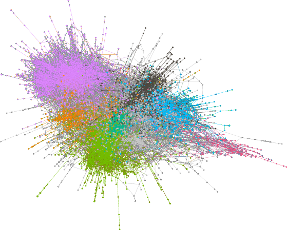
If you want to create our two network diagrams, you'll need one additional piece of software: Gephi, the Open Graph Viz Platform. We used it to generate Figure 2 in the chapter, a "hairball" network graph of the citation network in our dataset. Like all the software used here, it is free/open source software and available for download.
Gephi is a graphical and interactive tool so, unlike the rest of our analysis, it will take some clicking around to reproduce our graph exactly.
We created Figure 2 in the following way:
code/bibliometrics/g_sm.graphmlTo create the small network cluster in Figure 3:
code/bibliometrics/cluster.graphmlGetting things just right will take some fiddling! We've included our Gephi files (code/bibliometrics/clusters.gephi and code/bibliometrics/g_sm.gephi) which are finished or mostly finished versions that you can open up and use if you'd like.
The code/topic_modeling directory applies latent Dirichlet allocation(LDA) topic modeling to the social media abstracts.
LDA takes in a set of documents and produces a set of topics and a distribution of topics for each document. The first file takes in the abstract file, and creates two outputs: The abstracts together with their topic distribution and a set of topics and the top words associated with each.
Our topic modeling analysis includes the following steps:
Run the following Python script that extracts our topics:
python3 code/topic_modeling/00_topics_extraction.pyNote that this will take some time —5-10 minutes on a decent laptop.
Run a second file which (a) makes a couple of tables of the top words for each topic and (b) generates some summary statistics for how the topics change over time. These statistics are used, e.g., to create Figure 4. You can run this with:
python3 code/topic_modeling/01_make_paper_files.pyTopic modeling is a stochastic process, and you may notice differences—potentially large differences—between the results in our chapter and the results when you run it. If the order of topics has changed (or if you think other labels would be appropriate for some topics), then you can adjust the topic names by editing the topic_names list in the 01_make_papers.py file.
For the prediction analysis, we use features of the papers to predict whether or not a paper gets cited.
These commands require a computer with a large amount of memory (i.e., RAM). We had trouble running these steps on our laptops which did not have enough memory. If you don't have access to such a computer, then you can change the n_features variable in the 00_ngram_extraction.py file from 100000 to something like 3000. This will change how many terms are included in the prediction analysis, but shouldn't make an important difference in the results.
We ran the following steps:
Because one of the features we use is the text of the abstracts, we start by getting uni-, bi-, and tri-grams from the abstracts. This is done with the 00_ngram_extraction.py python file:
python3 code/prediction/00_ngram_extraction.pyThis will create an
ngram_table.csvfile in theprocessed_datadirectory.
Next, we build control variables:
Rscript code/prediction/01-build_control_variables.R This will build a set of descriptive variables, saved to
paper/data/prediction_descriptives.RData
Then, we create textual features using the ngram table we created:
Rscript code/prediction/02-build_textual_features.RThis step filters the ngrams to those which occur across 30 subject areas and saves them as a matrix at
processed_data/top.ngram.matrix.RData.
Finally, the data that we've collected is put into models, and statistics are collected:
Rscript code/prediction/03-prediction_analysis.RThis step will save the output of the models to
paper/data/prediction.RData.
Each of these final two steps will take a long time to run.
Now we should have all of the data that we need sitting in the paper/data directory. We use a package called knitr to load and manipulate data directly in the chapter. With the exception of the Gephi graphs, all of the tables and figures in the chapter are created using code that is in the same file where we write the text of the chapter. The knitr package is the magic behind the scenes that makes that possible.
To build the chapter, we will be using a Makefile which requires a set of utilities to run. This is the part that might get a little tricky for Windows users.
You can install the packages you'll need from Debian or Ubuntu with the following command:
apt install rubber latexmk texlive-latex-recommended texlive-latex-extra texlive-fonts-extra texlive-fonts-recommended texlive-bibtex-extra moreutils gawkAfter this, you should change to the paper directory and simply run the command make.
This will produce a quickly scrolling output to standard out, and if everything has worked, then in the end it will produce a bunch of files in the paper directory, one of which will be the final PDF file!
An alternative approach that does not involve installing software is to upload the entire paper subdirectory (including the paper/data subdirectory) as a paper repository to the service ShareLaTeX. In order to make it work, you'll also need to rename the file ending with .Rnw to .Rtex. We spent some of the time writing our paper using ShareLaTeX so this should work.
Although we have tried to make this document as clear as possible and although we have tested it ourselves, there are many ways it might fail. You might have a different software environment or the software dependencies we have used might have bit rot over time in a way that leads to things breaking.
You are welcome to get in touch with us if you have questions and we have provided our webpages and emails here for that purpose:
If you can fix issues you run into, find ways to clarify our instructions, or make fixes to our code, please tell us! We'd love to add helpful improvements to these materials.
In addition to the archival version in the Dataverse, we have hosted our code in a git revision control management repository here: https://code.communitydata.cc/social-media-chapter.git Even the page you are reading is included in our repository. If you notice any typos or errors, please send us your fix! To do so, you can follow the instructions we have posted for sending updated versions of our code or documentation. Your work and improvements can help others trying to replicate and learn from this project.